Error propagation

Overview

Three functions are used to study the error propagation from measured PV data to hydrogen based fuels techno-economic modeling:

• solve_optiplant()

• calculate_all_LCOF_diff()

• generate_LCOF_diff_plot()

Techno-economic assessment model

The function solve_optiplant() is used to perform an optimization of investments and operation for a hydrogen based fuel production system. More details about the model can be found in this article and repository.

Parameters

Name	Type	Description
data_units	pandas.DataFrame	Techno-economic parameters for all system units.
PV_profile	pandas.DataFrame	Hourly renewable generation profile.
H2_end_user_min_load	float	Minimum H₂ end-user load as a fraction of capacity.
solver_name	str	LP solver name (e.g., “GUROBI_CMD” or “PULP_CBC_CMD”).

Returns

Return	Type	Description
fuel_cost	float	Fuel production cost (EUR/t).
df_results	pandas.DataFrame	Summary of techno-economic results.
df_flows	pandas.DataFrame	Hourly flow and electricity data.

Notes

• Explicitly models storage, demand, and power balances.

• Includes investment annuities and maintenance periods.

• Uses PuLP for linear programming.

Example

(The file PV_profile.csv should be created by the user)

import pandas as pd
from simeasren import solve_optiplant

data_units = pd.read_csv("Techno_eco_data_NH3.csv")
pv_profile = pd.read_csv("PV_profile.csv")

fuel_cost, df_results, df_flows = solve_optiplant(
    data_units=data_units,
    PV_profile=pv_profile,
    H2_end_user_min_load=0.3,
    solver_name="GUROBI_CMD"
)
print(f"Fuel cost: {fuel_cost:.2f} EUR/t")

---

Calculate LCOF differences

calculate_all_LCOF_diff() calculates and compares Levelized Cost of Fuel (LCOF) differences between measured and simulated renewable profiles for all the simulated tools running the “OptiPlant” tool for each profile.

Parameters

Name	Type	Description
data_sim_meas	pandas.DataFrame	Combined measured and simulated data.
location_name	str	Location to analyze.
H2_end_user_min_load	float	Minimum load for H₂ end-user.
solver_name	str	LP solver name.
technoeco_file_name	str	Techno-economic data file (default: “Techno_eco_data_NH3”).

Returns List of dictionaries with:

• "Location" — Location analyzed.

• "Tool" — Simulation tool name.

• "LCOF Difference (%)" — Percentage deviation vs. measured data.

The results of the optimization (hourly optimal profiles, system sizing and costs) are saved as csv file in the results/location/Techno-eco assessment results folder for each PV power profile.

Example

from simeasren import calculate_all_LCOF_diff, prepare_pv_data_for_plots

data_sim_meas, _, _ = prepare_pv_data_for_plots("Utrecht", "2017")
results = calculate_all_LCOF_diff(
    data_sim_meas=data_sim_meas,
    location_name="Utrecht",
    H2_end_user_min_load=0.3,
    solver_name="GUROBI_CMD"
)
print(results[0])

---

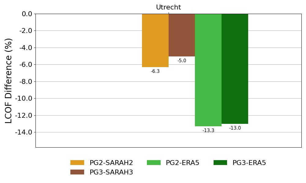
Plot LCOF differences

generate_LCOF_diff_plot() Generates a bar plot comparing LCOF differences between measured and simulated datasets across tools.

Parameters

Name	Type	Description
LCOF_diff_results	list[dict]	Output from calculate_all_LCOF_diff().
location_name	str	Location analyzed.
year	str	Year label for the plot.
H2_end_user_min_load	float	Hydrogen end-user load constraint.
output_root	str	Directory to save the plot (default: “results”).

Returns None (saves plot directly).

Example

from simeasren import generate_LCOF_diff_plot, calculate_all_LCOF_diff, prepare_pv_data_for_plots

data_sim_meas, _, _ = prepare_pv_data_for_plots("Utrecht", "2017")
results = calculate_all_LCOF_diff(data_sim_meas, "Utrecht", 0.3, "GUROBI_CMD")

generate_LCOF_diff_plot(
    LCOF_diff_results=results,
    location_name="Utrecht",
    year="2017",
    H2_end_user_min_load=0.3
)